HybriD3 Local Training Scaffold Test
Date: 2026-05-30
PDF version: hybrid3-local-training-scaffold-test.pdf
Summary
This local smoke study pulled ten similar HybriD3 atomic-structure records, cataloged their database and crystallographic metadata, generated a compact GIWAXS simulation set for 2D fibril-textured samples, applied detector-image artifacts, trained the baseline vector ranker, evaluated top-k recovery, and exported ranked structure-file guesses.
| Quantity | Value |
|---|---|
| Structures pulled | 10 |
| Clean simulation samples | 20 |
| Artifact-augmented samples | 80 |
| Missing-wedge corrected clean samples | 20 / 20 |
| Median missing-wedge masked fraction | 0.082 |
| Surface-artifact augmented samples | 60 |
| Ranker candidates | 20 |
| Evaluated artifact images | 80 |
| Solvable augmented fraction | 1.000 |
| Median artifact SNR | 13.49 |
| Top-1 accuracy | 0.988 |
| Top-5 accuracy | 1.000 |
Pulled Structure Cohort
Selection targeted visible HybriD3 atomic-structure datasets with 2D PbI4
lead-iodide inorganic sublattices. This gives a chemically coherent local test
set for fibril-textured GIWAXS recognition while keeping the run small.
| Dataset | Structure id | Inorganic | Organic | File | Sites |
|---|---|---|---|---|---|
| 2788 | hybrid3_2788 |
PbI4 | C4H9NI | dataset_2788_20231011_MC3I_PbI_380K_red.cif |
20 |
| 2787 | hybrid3_2787 |
PbI4 | C4H9NI | dataset_2787_20250421_MC3I_PbI_360K_1_red.cif |
20 |
| 2786 | hybrid3_2786 |
PbI4 | C4H9NI | dataset_2786_MC3PI_100K.cif |
20 |
| 2736 | hybrid3_2736 |
PbI4, Lead iodide | C7H9IN | dataset_2736_geometry.vasp |
82 |
| 2735 | hybrid3_2735 |
PbI4, Lead iodide | C7H9BrN | dataset_2735_geometry.vasp |
82 |
| 2734 | hybrid3_2734 |
PbI4, Lead iodide | C7H9ClN | dataset_2734_geometry.vasp |
82 |
| 2733 | hybrid3_2733 |
PbI4, Lead iodide | C7H9FN | dataset_2733_geometry.vasp |
164 |
| 2732 | hybrid3_2732 |
PbI4, Lead iodide | C6H18N2 | dataset_2732_geometry.vasp |
62 |
| 2731 | hybrid3_2731 |
PbI4, Lead iodide | C8H22N2 | dataset_2731_geometry.vasp |
74 |
| 2730 | hybrid3_2730 |
PbI4, Lead iodide | C2H8NO | dataset_2730_geometry.vasp |
58 |
Simulation Protocol
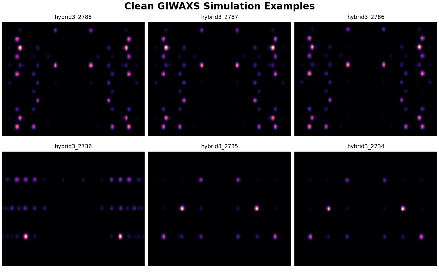
Clean GIWAXS images were generated on a deliberately lower-information
reciprocal-space grid with qxy = [-2.8, 2.8] A^-1, qz = [0.0, 2.8] A^-1,
and 160 x 128 local smoke-test pixels. The default cap is now biased toward
2-3 A^-1 rather than 4 A^-1 so the solver is tested against detector windows
that resemble practical GIWAXS measurements with less high-q information. The
texture model was fiber_gaussian with theta_x = 90 deg,
theta_y = 0/90 deg, sigma_theta = 0.035, sigma_phi = 0.28,
sigma_r = 0.04, q-dependent broadening terms of 0.25 in-plane and 0.15
out-of-plane, and hkl_extent = 14. The hkl extent is selected as the
maximum recommended reciprocal-lattice search across the pulled structures for
the requested q-range, so long-axis 2D structures such as hybrid3_2788,
hybrid3_2787, and hybrid3_2786 still populate the detector plane out to
q <= 2.8 A^-1.
The local forward model now includes a first-order flat-detector solid-angle
response derived from the Ewald-sphere scattering angle
q = 4 pi sin(theta) / lambda. This keeps the edge of the detector realistic
while preserving the existing labeled (hkl) peak table contract. The same
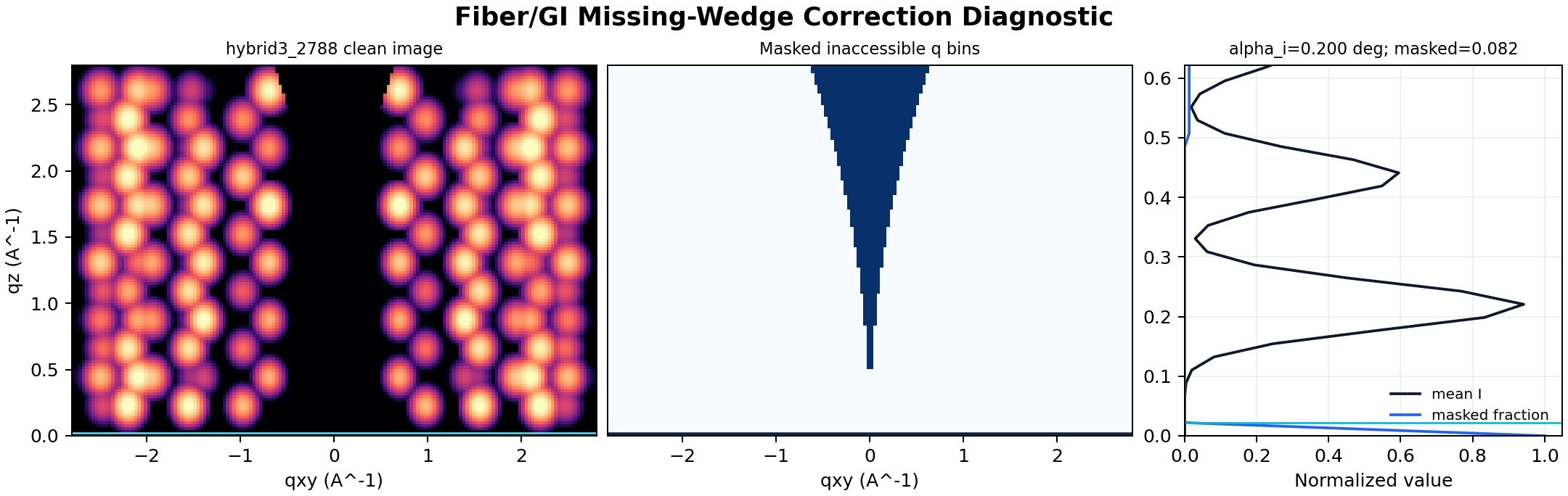
incident-angle geometry is also applied as a pyFAI-style fiber/GI missing-wedge
correction in qIP/qOOP space, so inaccessible bins below the sample horizon are
zeroed and excluded from the labeled (hkl) peak table. This run applied the
pyfai_fiber_qip_qoop_accessibility missing-wedge model to 20 of
20 clean samples, with a median horizon of
qz = 0.0219 A^-1 and a median masked fraction
of 0.082. Every generated clean label
stores a simulation_metadata block with the missing-wedge model, incident
angle, wavelength, horizon, and masked fraction used for the example.
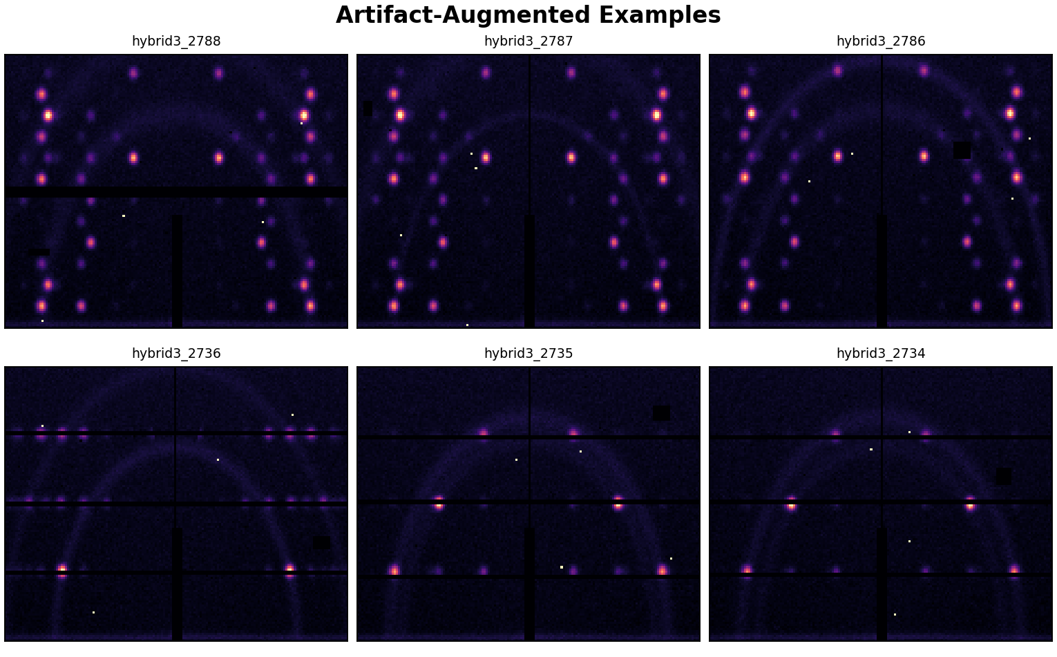
Detector artifacts were generated from the scaffold artifact profiles:
clean, default, harsh_detector, and pilatus1m_reference. Diffuse
scattering is now generated as broad rings centered on q-values inferred from
the simulated Bragg signal, instead of arbitrary vertical detector streaks.
The profiles also include Poisson noise, Gaussian read noise, q-dependent
background, direct/specular beam artifacts, Yoneda bands, substrate horizon
shadowing, critical-angle peak splitting, beamstop shadow, flat-field variation,
hot/dead pixels, dead-pixel clusters, saturation, and detector-module masks
scaled from randomized common detector footprints including PILATUS 1M, EIGER2,
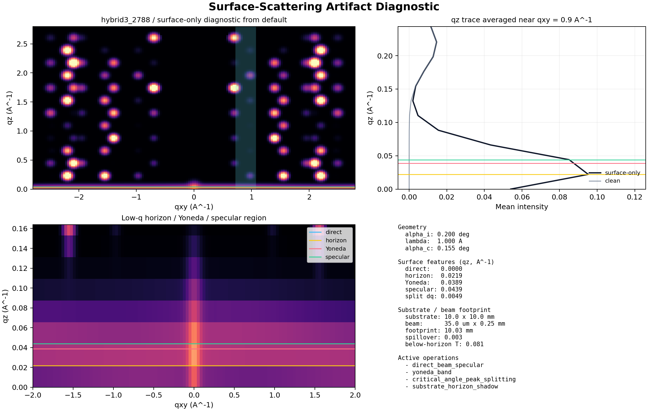
and a continuous PerkinElmer-style flat panel. The direct-beam, Yoneda,
horizon, and critical-angle operators use the same incident angle and wavelength
stored in the detector geometry. The critical angle is estimated from the parsed
structure electron density unless a profile overrides it. The substrate horizon
model computes beam-footprint spillover from substrate dimensions, beam
width/height, and incident angle, then uses that spillover to tune the horizon
shadow, below-horizon leakage, and added qz peak broadening. The active
surface-scattering operations in this example are direct_beam_specular, yoneda_band, critical_angle_peak_splitting, substrate_horizon_shadow, footprint_spillage_peak_broadening. Each
artifacted label now includes an artifact_assessment block that turns direct
beam, specular reflection, Yoneda bands, substrate horizon/footprint spillage,
critical-angle peak splitting, beamstop shadows, and detector masks into compact
q-space or pixel-space regions. The feedback evaluator and exported structure
guesses rasterize those regions into artifact-aware ranking weights and blend
them with the clean image-overlap score, so non-Bragg aberrations are recognized
without discarding the Bragg-rich regions needed for peak assessment/indexing
tests.
The mathematical surface-artifact contract and artifact-aware training model are documented in Surface Artifacts And Training Model.
The augmentation quality gate records quality_assessment for every label. In
this smoke run, 80 of 80 artifacted
samples are marked solvable, with a median signal-to-noise of
13.49 and a median retrievable-signal fraction of
1.000. The harsh profile is kept as
a controlled stress-test tail, but its noise, saturation, horizon
spillover, direct-beam, and diffuse-ring strengths are bounded so it remains a
recoverable indexing problem rather than an unrealistic failure case.
Simulation Examples
Output Locations
| Output | Path |
|---|---|
| Run root | /Users/keithwhite/repos/ewald/data_training/runs/hybrid3_2d_fibril_smoke_20260530 |
| HybriD3 catalog | /Users/keithwhite/repos/ewald/data_training/runs/hybrid3_2d_fibril_smoke_20260530/hybrid3_library/hybrid3_structure_catalog.yaml |
| Ingest manifest | /Users/keithwhite/repos/ewald/data_training/runs/hybrid3_2d_fibril_smoke_20260530/hybrid3_library/hybrid3_ingest_manifest.jsonl |
| Clean simulation manifest | /Users/keithwhite/repos/ewald/data_training/runs/hybrid3_2d_fibril_smoke_20260530/simulations/manifest.jsonl |
| Artifact manifest | /Users/keithwhite/repos/ewald/data_training/runs/hybrid3_2d_fibril_smoke_20260530/artifacts/artifact_manifest.jsonl |
| Ranker model | /Users/keithwhite/repos/ewald/data_training/runs/hybrid3_2d_fibril_smoke_20260530/model/vector_ranker.json |
| Feedback metrics | /Users/keithwhite/repos/ewald/data_training/runs/hybrid3_2d_fibril_smoke_20260530/metrics/feedback_metrics.json |
| Exported guesses | /Users/keithwhite/repos/ewald/data_training/runs/hybrid3_2d_fibril_smoke_20260530/structure_guesses |
Testing Protocol
- Verify HybriD3 REST access and select ten visible 2D
PbI4atomic-structure datasets. - Download structure-like files from HybriD3 dataset pages and JSmol media endpoints.
- Convert supported structure variants to simulator-readable CIF/POSCAR files.
- Write an enriched EWALD structure catalog with API metadata and file-derived crystallographic metadata.
- Generate clean GIWAXS simulations using the 2D fibril-texture sweep and
verify the
simulation_metadata.missing_wedge_correction_appliedlabels. - Apply deterministic detector and surface-scattering artifacts, then verify
artifact_metadata.operations,artifact_assessment.regions, andquality_assessment. - Build the baseline vector-ranker checkpoint from clean simulations.
- Evaluate artifact images against the ranker and export top-k structure-file guesses for downstream structure-analysis testing.
Detector And Literature Basis
- The PILATUS 1M reference mask follows published modular-detector behavior: the original 18-module detector has a large pixel array, module gaps, and measurable non-responding pixels that must be masked or treated during data reduction.
- The pyFAI detector database provides practical detector definitions and masks for many common X-ray detectors, including PILATUS, EIGER, PerkinElmer, Rayonix, Lambda, Jungfrau, and other beamline detector families.
- The EIGER2 detector profiles use the DECTRIS-published 75 um pixel size and inter-module gap patterns for EIGER2 X detector geometries.
- The GIWAXS protocol follows the perovskite-oriented guidance in Steele et al., "How to GIWAXS: Grazing Incidence Wide Angle X-Ray Scattering Applied to Metal Halide Perovskite Thin Films," Advanced Energy Materials 2023, 13, 2300760, including attention to q-range, grazing-incidence geometry, detector mapping, and orientation-sensitive interpretation.
References:
- Broennimann et al., "The PILATUS 1M detector," https://journals.iucr.org/s/issues/2006/02/00/gf0003/
- pyFAI detector distortion and detector-definition documentation, https://pyfai.readthedocs.io/en/latest/usage/tutorial/Detector/Distortion/Distortion.html
- DECTRIS EIGER2 X/XE detector specifications, https://www.dectris.com/en/detectors/x-ray-detectors/eiger2/eiger2-for-synchrotrons/eiger2-x/
- Steele et al., Advanced Energy Materials 2023, DOI 10.1002/aenm.202300760, https://doi.org/10.1002/aenm.202300760
Interpretation
This is a scaffold validation, not a final scientific model benchmark. The baseline vector ranker is intentionally simple: it tests whether the data contracts, labels, manifests, image generation, artifact augmentation, and structure-guess export are connected. The next technical step is to replace the baseline ranker with a learned peak-detection/indexing/retrieval model while keeping the same manifest and reporting contracts.